How to create short-term and long-term forecasting?

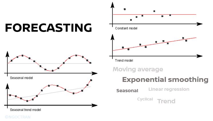
Published by Ngoc Tran on 25 September 202325 September 2023

Figure 1. Forecasting (made by the author)

Imagine if your manager requests you to create an inventory forecast for next month, how would you do that? Or how do you make a forecast to evaluate if there is sufficient budget for a supplier until the end of the year? Meanwhile, it happens to you that there is no available computer-generated forecast… Don’t worry! Let’s have a look together at the following forecasting techniques that may help answer your questions.

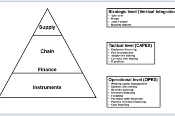
First, let’s understand that forecasting can be used for making various decisions, for example, estimation of the need for more supplier capacity, budgeting, demand, expansion, etc. For different levels of decisions (e.g. strategic, tactic, operational), it requires an applicable forecasting method, together with other factors such as level of aggregation, forecast frequency, the amount of top management involvement, and length of the forecast.

Now, we can discover which forecasting techniques are suitable for short-term and intermediate/long-term periods. Short-term forecasting can be done daily, weekly or monthly. Intermediate/long-term forecasting can be done quarterly, yearly, or longer.

#1: Short-term forecasting techniques

The techniques shown in Figure 2 are often used in inventory control, inventory planning, and monthly demand.

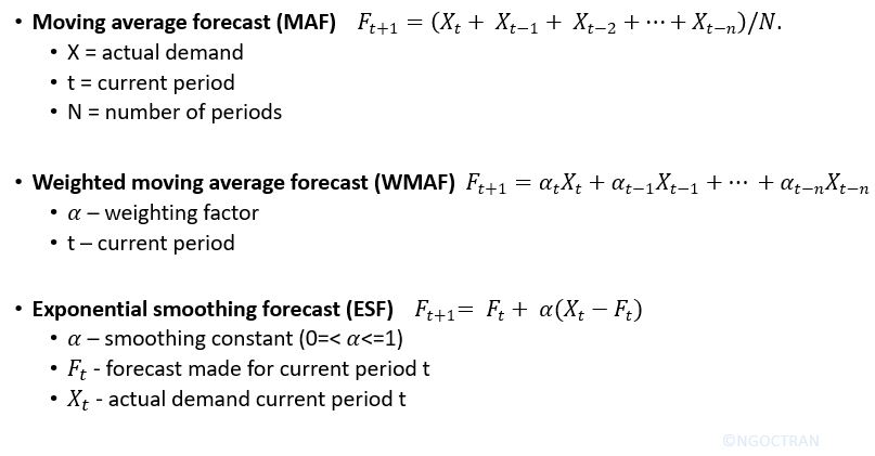
Figure 2. Short-term forecasting equations (made by the author)

The moving averages and exponential smoothing are two common short-term forecasting methods:

Moving average averages past demand to project a forecast for future demand, often for the next few periods. The goal is to smooth out the random fluctuations while considering any possible changes within the time period. Because of this technique’s nature, it’s better to use recent data rather than ones that are several months or years old.
Weighted moving average While the moving average assigns the same weight to each period, the weighted moving average model assigns different weights to each period. The more recent the period, the higher the weight. The sum of the weights must total 100%.
Exponential smoothing projects a forecast by using the most recent data. This forecast is made at the end of period N for period N + X in the future. Lookng at the formula in figure 2 above, the higher the smoothing constant is, the more responsive forecasts are to changes and vice versa.

Note: According to F. Robert Jacobs et al. (2011), simple forecasting performs better than the more complicated ones for detailed forecasts, especially over short periods. Besides, it’s highly recommended to take into account demand and supply patterns while creating the forecast. For example, are there any special promotions or advertising in place? What are currently your competitors’ actions?

#2: Intermediate-term forecasting techniques

There are linear regression forecasting and cyclic decomposition techniques that help determine the underlying trends based on historical values. Specifically, these techniques look into historical data to understand how different variables impact others. From there, they develop an algorithm to forecast in an intermediate to a long-term period.

Linear regression: refers to the special class of regression where the relationship between variables (data) forms a straight line Y = a + bx. It is commonly used for long-term forecasting like forecasting the demands of product families. However, the biggest restriction of this method is that it assumes past data and future projects fall about a straight line, meaning that projected data tends to increase/decrease over time. You can plot your data in Excel, then create a line chart and select “Display equation on chart” in ‘Format Trendline” to obtain the regression equation.
Cyclic decomposition: separates the time series data into different components of demand: trend, seasonal, and cyclical. The benefit of this method is that it’s easy to see the outliers when a forecast is de-seasonalized. When demand contains both seasonal and trend effects, there are two types of seasonal variations:
- Additive seasonal variation: applies when the seasonal amount is constant no matter what the trend is. It is calculated by the sum of Trend and Seasonal factors.
- Multiplicative seasonal variation: opposite to the one above, indicating when there are multiplicative seasonal variations. It is therefore calculated by the product of Trend and Seasonal factors. This method is regularly used in practice. However, due to its complexity, you can follow my next post about how to create this kind of forecast based on an example.

One of the last concerns would be “How accurate is my forecast?”. In general, in the beginning, you can try out different methods at the same time and reflect on the results. For the short-term forecast, you can closely monitor the forecast and analyze the difference between the forecast and the actual. Besides, forecast bias can be among the techniques for evaluating the forecast quality. For more information, you can read it via this link.

Thank you for reading and please share if you find it useful!

How to create short-term and long-term forecasting?

How to create a seasonal trend forecast?