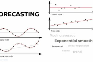
Following up on my previous post about forecasting, this post focuses on creating a seasonal trend forecast by using the decomposition of time series data as it indicates a non-linear trend, meaning that it can display changes that fluctuate over time. These changes can be seen as changes in demand and supply.

In general, decomposition of time series data can be done as follows:

Step 1: Find the seasonal factor

• Determine average actual demand per specific period (e.g., per month). For example, if actual demand data for Jan, Feb, and Mar 2022 are 10, 20, and 30 respectively, then the average actual demand per month is (10+20+30)/3 = 20.
• Determine average total actual demand (e.g., per year)
• Calculate seasonal factor: average actual demand/ average total actual demand. For example, actual demand in Jan 2022, and Jan 2023 are 15, and 17 respectively. Then, the average actual demand for Jan (15+17)/2 = 16. The average total actual demand from Jan 22 to Jan 23 is 100. The seasonal factor for Jan is calculated as follows: 16/100 = 0.16

Step 2: Create a simple linear regression model by de-seasonalized demand

• De-seasonalized actual demand per specific period based on the seasonal factor (this means taking the seasonal factor out of your actual demand) = actual demand/ seasonal factor
• Use linear regression (Excel) to fit trend line to de-seasonalized data

Step 3: Create a seasonal trend forecast

Calculate forecast demand per specific period (e.g., per month).

The formula is (y= a + bx) * seasonal factor, where y = a + bx is the linear regression and x is the period number (see an example of period numbers in Figure 1).

Example: If you have y = 20 + 10x and seasonal factor is 0.5, then the forecast in period x = 10 is calculated as y = (20 + 10*10)*0.5 = 60

Let’s look at the example below to see how the seasonal trend forecast can be calculated. The example shows the actual demand per month from 2022 to 2023 for company A. The goal is to prepare a forecast for next year.

Figure 1. Forecast example (made by the author)

To find the seasonal factor, we first need to determine the average actual demand per month. The example shows data for two years, so the average actual demand per month is the sum of actual demand for Month X/2022 and Month X/2023 divided by the number of months. For example, the average actual demand of January = (800 + 980)/2. The same calculation applies to the rest of the data. Then, we calculate the average total actual demand in two years, which is the sum of actual demand in all periods divided by the number of periods (in this case, 20 periods). Following the last formula in step 1, we obtain the seasonal factor (e.g., seasonal factor for January = 890/2117). Please refer to Figure 2 (steps 1.1 to 1.3) for all calculations.

Figure 2. Calculations based on the example (made by the author)

Moving to step 2, we take the average actual demand per month divided by the corresponding seasonal factor. Please refer to step 2.1 in Figure 2. The results are de-seasonalized actual demand, which we will use to create a simple linear regression. In Excel, select the data and insert chart type X Y (Scatter), and right-click in the chart to choose “Add Trendline”. By right-clicking on the trend line and selecting “Format Trendline”, scroll down and select “Display Equation on chart”. Now, you have the equation of the data trend, which is y = 35.765x + 1741.5.

Finally, we create a de-seasonalized trend forecast for the coming year. Since x in the equation is the number of a period, you need to continue counting the period number of the coming months. For instance, actual demand stops at 20, so the period number is 21 for Sep 2023, 22 for Oct 2023, and so on. Then, we multiply the forecast per period with the corresponding seasonal factor. Figure 3 displays the forecast for next year.

Figure 3. Seasonal trend forecast for next year based on historical data from the example (made by the author)

Besides this technique, it’s worth trying to use the seasonal factor in other forecasting formulas like simply playing with the numbers and comparing different results. How about multiplying the seasonal factor with the result from the moving average forecast technique? Or with an exponential smoothing forecasting method? Would it get you closer to the actual demand?

In short, the decomposition of time series data technique helps you to gain an overview of fluctuations over a period of time.

Thank you for reading! Please share if you find this article useful!

Recommended reading:

Manufacturing planning and control for supply chain management (F. Robert Jacobs et al., 2011)

https://machinelearningmastery.com/decompose-time-series-data-trend-seasonality/

https://otexts.com/fpp2/decomposition.html

Series Forecasting